EWAS Analysis in MVP
2024-12-02
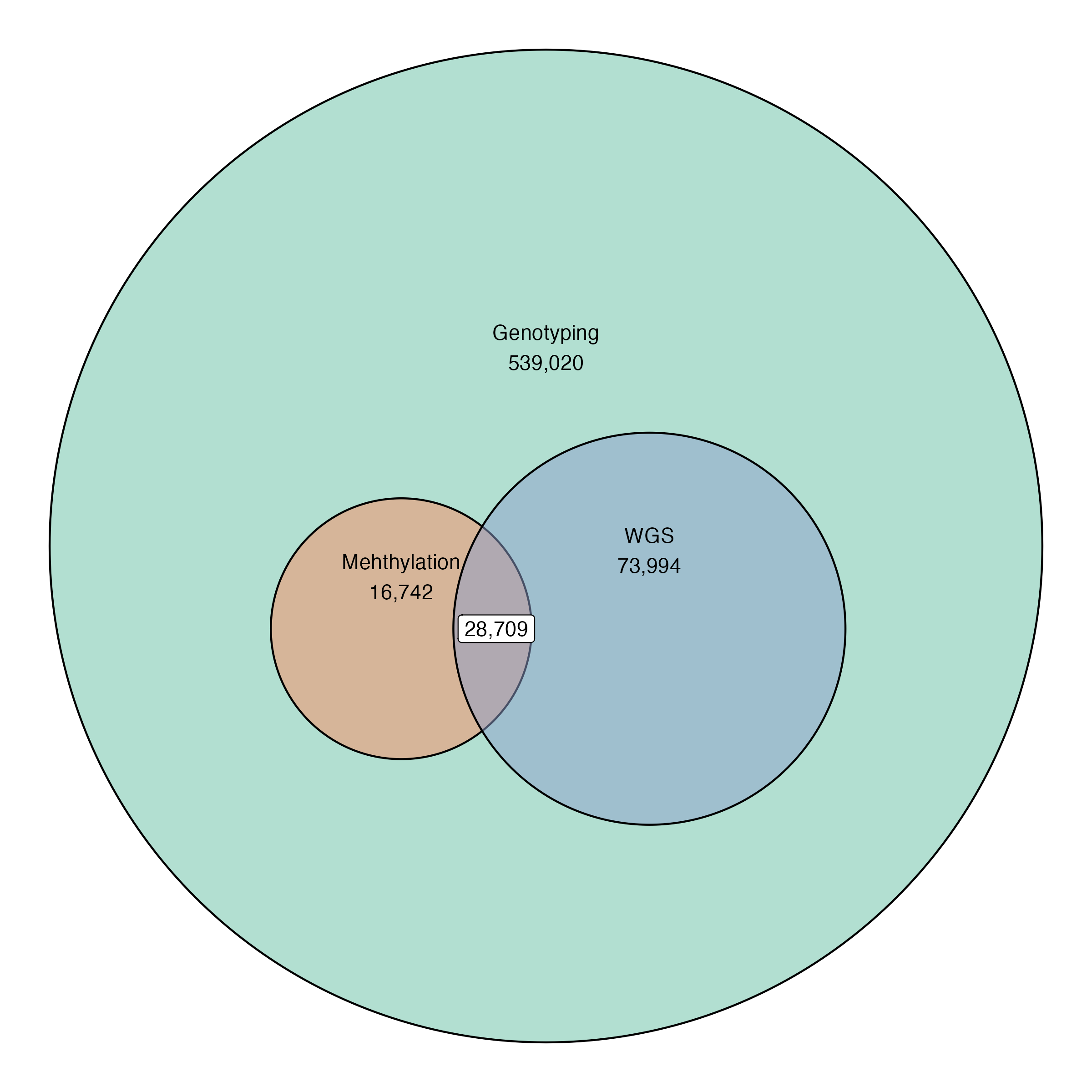
Million Veteran Program
Current data release:
539,020 Individuals
28,709 (~64%) with whole genome sequencing
45,460 individuals with methylation data
Among these, ~40% are T2D.
Problem Setting
Assume we have \(N\) subjects, \(d\) covariates (including the intercept), and \(M\) CpG sites or probes. EWAS requires repeatedly estimating the model:
\[ \boldsymbol{\beta}_j \sim \mathbf{x}\alpha_j + \mathbf{Z}\boldsymbol{\gamma}_j + \boldsymbol{\epsilon}_j \]
where \(\epsilon_{ij} \sim \mathrm{N}(0, \sigma_j^2)\) for \(j = 1, \dots, M\). The regression coefficients \(\alpha_j\) are the parameters of interest, and parameters \(\boldsymbol{\gamma}_j\) are nuisance parameters. Concatenating the \(M\) regression models together, we have:
\[ \boldsymbol{B} \sim \mathbf{x}\boldsymbol{\alpha}^\top + \mathbf{Z} \boldsymbol{\Gamma} + \mathbf{E} \]
Let \(\boldsymbol{\Theta} = [\boldsymbol{\alpha} : \boldsymbol{\Gamma}^\top]^\top\) and \(\mathbf{W} = [\mathbf{x} : \mathbf{Z}]\). The least squares estimates are straightforward: \[ \widehat{\boldsymbol{\Theta}} = \left(\mathbf{W}^\top \mathbf{W}\right)^{-1} \mathbf{W}^\top \boldsymbol{B} \]
and \(\widehat{\sigma}_j^2 = \frac{1}{n-d}\sum_{i=1}^N b_{ij} - \mathbf{w}_i^\top \widehat{\boldsymbol{\theta}}\).
In the case of MVP, we have roughly \(M \approx 750,000\) and \(N \approx 45,000\), which would require over 250 Gb of memory to store all at once.
Methylation Data in MVP
In MVP, \(\boldsymbol{\beta}_1, \dots, \boldsymbol{\beta}_M\) have been stored in the HDF5 file format, which stores each chromosome as a separate table. Suppose we have an arbitrary chromosome \(\mathbf{B}^k\).
\[ \mathbf{B}^k = \begin{bmatrix} \mathbf{B}_{1,1}^k & \cdots & \mathbf{B}_{1, m_k}^k\\ \vdots & \ddots & \vdots\\ \mathbf{B}_{n_k,1}^k &\cdots &\mathbf{B}_{n_k, m_k}^k \end{bmatrix} \]
The chromosome with the largest amount of data, chromosome 1, is stored in 8 chunks, where the largest chunks are square matrices roughly 4 Gb in size (\(n_1 = 4,\, m_1 = 2\)).
The HDF5 file format stores each submatrix \(\mathbf{B}_{i, j}^k\) as a contiguous chunk in storage,
Access to any data stored within a particular chunk requires decompressing the entire chunk.
- Generally, decompression is a very slow operation, if possible, we would like to never decompress any chunk more than once.
Sufficient Statistics
Fortunately, the problem structure of EWAS almost lets us do this exactly, the regression coefficients estimates \(\widehat{\boldsymbol{\Theta}}\) only require:
The Gram matrix \(\mathbf{X}^\top \mathbf{X}\)
The \(d\) by \(M_k\) matrix product \(\mathbf{X}^\top \mathbf{B}^k\)
- \(d << N\) so we have no problems allocating the full array in-memory
Taking a closer look, we can represent \(\mathbf{X}^\top \mathbf{B}^k\) as summation,
\[ \mathbf{X}^\top \mathbf{B}^k = \begin{bmatrix} \sum_{i=1}^{n_k} \mathbf{X}_i^\top \mathbf{B}_{i, 1}^k & \cdots & \sum_{i=1}^{n_k} \mathbf{X}_i^\top \mathbf{B}_{i, n_k}^k \end{bmatrix} \]
The term \(\sum_{i=1}^{n_k} \mathbf{X}_i^\top \mathbf{B}_{k, i, j}\) only depends on the \(j\)-th block column slice of \(\mathbf{B}\). Thus, we have exactly what we wanted, and only need to access one chunk of \(\mathbf{B}^k\) at a time.
Handling missing values in \(\mathbf{B}^k\) complicates this, but in the simple case of mean imputation, we still only need to store \(n_k\) chunks simultaneously.
For inference, we also require storing the residual sums of squares for each column, but this is only a vector of length \(M_k\)
Existing Implementation
The script EWAS.R in GENISIS is implemented using the meffil and bacon R packages, but in particular meffil does not take advantage of the inherent structure in the problem.
The default data access is in column slices of width \(5,000\), this requires decompressing every chunk up to 9 times due to a mismatch in how the \(\beta\) values are stored on-disk.
meffilmakes an empirical Bayes adjustment for the standard error \(\mathrm{SE}[\widehat{\alpha}_j]\), but in large sample sizes, this adjustment is unncessary.- This adjustment is also subtly incorrect when passing \(5,000\) sites at a time, and may induce bias in EWAS test statistics
Tries to load an entire chromosome into memory at a time, which is generally infeasible
baconconstructs a 3-component mixture approximation to the empirical null distribution of the test statistics but only depends on summary statistics, so it is quite fast
New Implementation
Only accesses at most 2 chunks simultaneously avoids high memory requirements
Peak memory usage is approximately 25 Gb for full EWAS on BMI
Longest job submission only takes 15-20 minutes to run EWAS on Chromosome 1 (the largest number of probes)
Parallel job submission over all chromosomes only takes 15-20 minutes, i.e. the time it takes for the longest running job to finish
Estimation of the empirical null using
baconcan be done by aggregating per chromosome summary statistics
EWAS for BMI
EWAS for BMI was conducted separately for the EUR and AFR self-reported ancestry, as well as all MVP subjects pooled together.
EUR: \(N = 27,137\)
AFR: \(N = 11,361\)
All MVP: \(N = 44,850\)
Model:
\[ \begin{aligned} \beta &\sim \text{BMI} + \text{sex} + \text{age} + \text{age}^2 + \text{cell composition(Houseman)}\\ &\qquad + \text{Scanner ID} + \text{Duration of Sample Storage}\\ &\qquad + \text{Technical PCs} + \text{Genomic PCs} \end{aligned} \]
EWAS for Glycemic Exposure
Hypothesis: HbA1c has a cumulative effect on DNA methylation levels
EWAS covariates of interest: historical HbA1c level 5 years prior to DNA methylation sample collection:
Sample Size: \(N = 13,567\)
Model:
\[ \begin{aligned} \beta &\sim \text{Mean HbA1c} + \text{sex} + \text{age} + \text{age}^2 + \text{cell composition(Houseman)}\\ &\qquad + \text{Scanner ID} + \text{Duration of Sample Storage}\\ &\qquad + \text{Technical PCs} + \text{Genomic PCs} \end{aligned} \]
Further Analysis
Complete case analysis instead of mean-imputation
Stratify by baseline or pre-baseline HbA1c level
Intensive treatment during DCCT resulted in an average of 7.0% HbA1c over the entire trial
Convential treatment during DCCT resulted in an average of 9.0% HbA1c over the entire trial
However, patients were randomized to each condition, which may not be comparable to MVP cohort
Stratify by race/ethnicity
- The sample in DCCT was 96% Caucasian, which is very different from MVP
Stratify by relative time of diagnosis with Type 2 diabetes (recently diagnosed vs. not recently diagnosed)
References
Footnotes
One subject was excluded due to large differences in estimated white blood cell composition.