Notes on High Dimensional Mediation Analysis
\[ \newcommand\indep{\mathrel{\perp\mkern{-11mu}\perp}} \newcommand\d{\mathrm{d}} \DeclareMathOperator{\EE}{\mathbb{E}} \DeclareMathOperator{\Pr}{\mathrm{Pr}} \newcommand{\<}{\left} \renewcommand{\>}{\right} \]
1 High-Dimensional Mediation Analysis
1.1 Model Formulation

Assume we have \(n\) independent observations from \(\<(A, M^{(1)}, \dots, M^{(p)}, Y, Z_M, Z_Y\>)\). Where,
\(A\) is the (univariate) exposure of interest,
\(M^{(1)},\,\dots,\,M^{(p)}\) are \(p\) possible mediators (CpG sites),
\(Y = \log(T)\) and \(T\) is a right-censored time-to-event outcome,
\(Z_M\) are \(q_M\) known confounders of the relationship between \(A\) and \(M\)
and \(Z_Y\) are \(q_Y\) confounders of the relationship between \(A, M\) and \(Y\).
1.1.1 Univariate Mediation Analysis

It is helpful to consider the single mediator case before considering the multiple-mediation problem. For any subject \(i\) and a specific mediator \(M^{(k)}\), we have the model,
\[ \begin{align} m_i^{(k)} &= \beta_0^{(k)} + \beta_A^{(k)} a_i + \mathbf{z}_{M,i}^\top \boldsymbol{\beta}_M^{(k)} + \varepsilon_i^{(k)} \\ y_i &= \theta_0^{(k)} + \theta_A^{(k)} a_i + \theta_M^{(k)} m_i^{(k)} + \mathbf{z}_{Y,i}^\top \boldsymbol{\theta}_Y^{(k)} + \sigma^{(k)} \xi_i^{(k)} \end{align} \]
where \(\varepsilon_1^{(k)}, \dots, \varepsilon_n^{(k)}, \xi_1^{(k)}, \dots, \xi_n^{(k)}\) are independent error terms. Collecting all \(n\) observations and omitting the index \(k\), the marginal effect of exposure \(A\) on \(Y\) mediated by \(M^{(k)}\) can be estimated by fitting two regression models:
\[ \begin{align} \mathbf{m} &= \mathbf{1}_n \beta_0 + \mathbf{a} \beta_A + \mathbf{Z}_M \boldsymbol{\beta}_M + \boldsymbol{\varepsilon}\\ \mathbf{y} &= \mathbf{1}_n \theta_0 + \mathbf{a} \theta_A + \mathbf{m} \theta_M + \mathbf{Z}_Y \boldsymbol{\theta}_Y + \sigma \boldsymbol{\xi} \end{align} \tag{1}\]
The estimate of marginal indirect effect, is defined by the product method estimator \(\beta_A \theta_M\). This implies that the null hypothesis of zero-mediation is,
\[ \begin{aligned} \mathrm{H}_0 &: \beta_A \theta_M = 0 &\equiv && \beta_A = 0 \text{ or } \theta_M =0 \end{aligned} \]
1.1.2 Marginal Hypothesis Testing
This is an instance of a composite null hypothesis, where the null hypothesis can be expressed as the union of three disjoint hypotheses, \(\mathrm{H}_0 = \mathrm{H}_{01} \cup \mathrm{H}_{10} \cup \mathrm{H}_{00}\).
\[ \begin{aligned} \mathrm{H}_{10}&: {\beta_A \neq 0} \wedge {\theta_M = 0}\\ \mathrm{H}_{01}&: {\beta_A = 0} \wedge {\theta_M \neq 0}\\ \mathrm{H}_{00}&: {\beta_A = 0} \wedge {\theta_M = 0}\\ \end{aligned} \]
1.1.2.1 A Wald-type test
The standard delta method approach is to take a normal approximation about the estimate \(\widehat{\beta}_A \widehat{\theta}_M\). The standard error of the estimated mediation effect is approximated by,
\[ \begin{aligned} \widehat{\operatorname{SE}}\<[\widehat{\beta}_A \widehat{\theta}_M\>] &= \sqrt{\widehat{\beta}_A^2 \widehat{\operatorname{Var}}[\widehat{\theta}_M] + \widehat{\theta}_M^2 \widehat{\operatorname{Var}}[\widehat{\beta}_A]} \end{aligned} \]
the covariance term is omitted, assuming \(\widehat{\beta}_A\) is independent of \(\widehat{\theta}_M\). Using this delta-method approximation gives the test statistic,
\[ T_{\mathrm{Sobel}} = \frac{\widehat{\beta}_A \widehat{\theta}_M}{\sqrt{\widehat{\beta}_A^2 \widehat{\operatorname{Var}}[\widehat{\theta}_M] + \widehat{\theta}_M^2 \widehat{\operatorname{Var}}[\widehat{\beta}_A]}} \]
this is known as the Sobel test of mediation. Liu (Liu et al. 2022) proved that, under the hypotheses \(\mathrm{H}_{10}\) and \(\mathrm{H}_{01}\), the test statistic \(T_{\mathrm{Sobel}}\) converges to a standard Gaussian asympototically. However, under \(\mathrm{H}_{00}\), \(T_{\mathrm{Sobel}}\) converges to \(\mathrm{N}\<(0, \frac 1 4\>)\). If we compare against a standard normal, that means that the test statistic will always be conservative under \(\mathrm{H}_{00}\). Furthermore, Liu also showed that for small \(\beta_1\) or small \(\theta_2\), Sobel’s test is conservative in finite samples.
1.1.2.2 The joint significance test
Alternatively, another way to approach testing for a mediation effect is by conducting a joint test that both \(\beta_A\) and \(\theta_M\) are non-zero. This defines the \(\mathrm{MaxP}\) test statistic, also referred to as the JS-uniform test statistic by Dai (Dai, Stanford, and LeBlanc 2022),
\[ T_{\mathrm{MaxP}} = \max\{p_{\beta_A},\, p_{\theta_M}\} \]
where \(p_{\beta_A}\) and \(\, p_{\theta_M}\) are the marginal p-values for testing whether \(\beta_A\) and \(\theta_M\) are equal to zero. Similar to the Sobel test, Liu showed that under \(\mathrm{H}_{01}\) and \(\mathrm{H}_{10}\), \(\mathrm{MaxP}\) is correctly uniformly distributed. Unfortunately, under \(\mathrm{H}_{00}\), the probability of rejecting the null at significance level \(\alpha\), is
Note that an equivalent test can be conducted by definining a test statistic \(T = \min\{|Z_{\beta_A}|, |Z_{\theta_M}|\}\) where \(Z_{\cdot}\) refers to the regression t-test statistic.
\[ \operatorname{Pr}\<[\mathrm{MaxP} < \alpha\>] = \operatorname{Pr}\<[p_{\beta_A} < \alpha\>] \times \operatorname{Pr}\<[p_{\theta_M} < \alpha\>] = \alpha^2 < \alpha \]
Thus, the \(\mathrm{MaxP}\) test is always conservative under \(H_{00}\), and only asymptotically consistent under \(\mathrm{H}_{10}\) and \(\mathrm{H}_{01}\). Even though the Sobel test and MaxP test are both conservative, Liu proved that the MaxP test is uniformly more powerful than the Sobel test.
1.1.2.3 Resampling-approaches
1.1.2.3.1 Non-parametric Bootstrap
As for the bootstrap, (Barfield et al. 2017), showed that under \(\mathrm{H}_{00}\), the non-parametric bootstrap based test is also overly conservative. Barfield considered 3 cases, corresponding to \(\mathrm{H}_{01}\), \(\mathrm{H}_{10}\), and \(\mathrm{H}_{00}\), respectively. Note that Barfield denoted confounders by \(X\) rather than \(Z\).
Case 1: no association between \(A\) and \(M\), but association between \(M\) and \(Y\), given \(A\) and \(X\): \(\beta_A = 0\); \(\theta_M \neq 0\);
Case 2: association between \(A\) and \(M\), but no association between \(M\) and \(Y\), given \(A\) and \(X\): \(\beta_A \neq 0\); \(\theta_M = 0\);
Case 3: no association between \(A\) and \(M\) and no association between \(M\) and \(Y\), given \(A\) and \(X\): \(\beta_A = 0\); \(\theta_M = 0\);
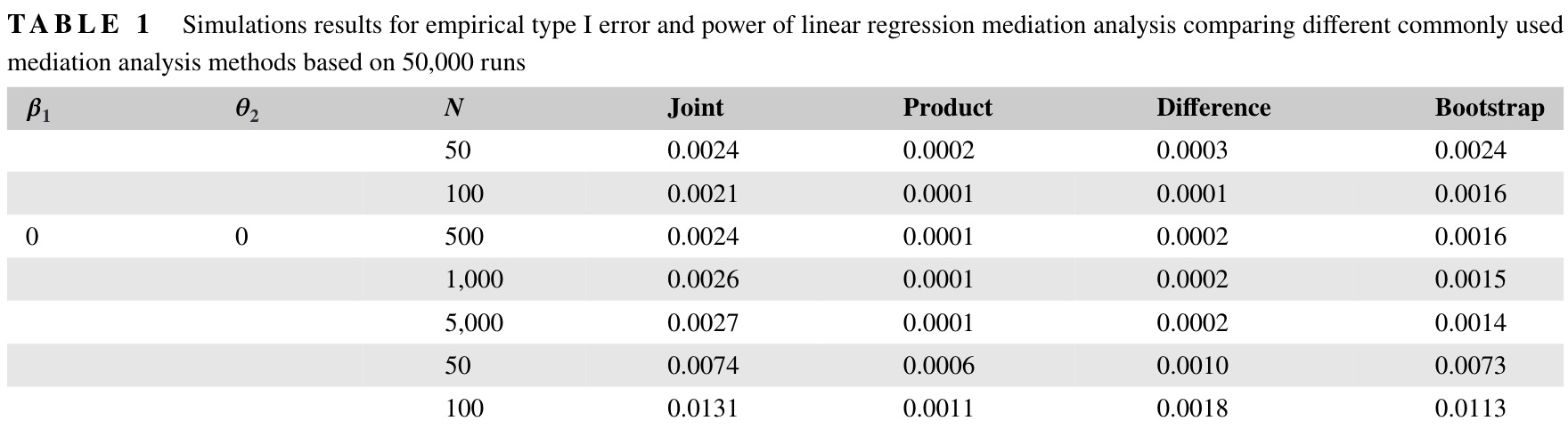
Under \(\mathrm{H}_{00}\), the \(\mathrm{MaxP}\) test had close to the expected Type-I error rate \(\alpha^2 = 0.05^2 = 0.0025\). All methods were conservative and had Type-I error well under \(\alpha=0.05\), including the bootstrap. Not shown are results corresponding to \(\mathrm{H}_{10}\), \(\mathrm{H}_{01}\), and \(\mathrm{H}_{11}\), In those situations, all methods had correct Type-I error and under \(\mathrm{H}_{11}\), high power
1.1.2.3.2 Adaptive Bootstrap
He (He, Song, and Xu 2024) attempted to remedy this by proposing an adaptive bootstrap algorithm, but simulations by Yang (Yang et al. 2025) show that when either \(\beta_A\) or \(\theta_M\) are small, the proposed adaptive bootstrap is anti-conservative and fails to control Type-I error.
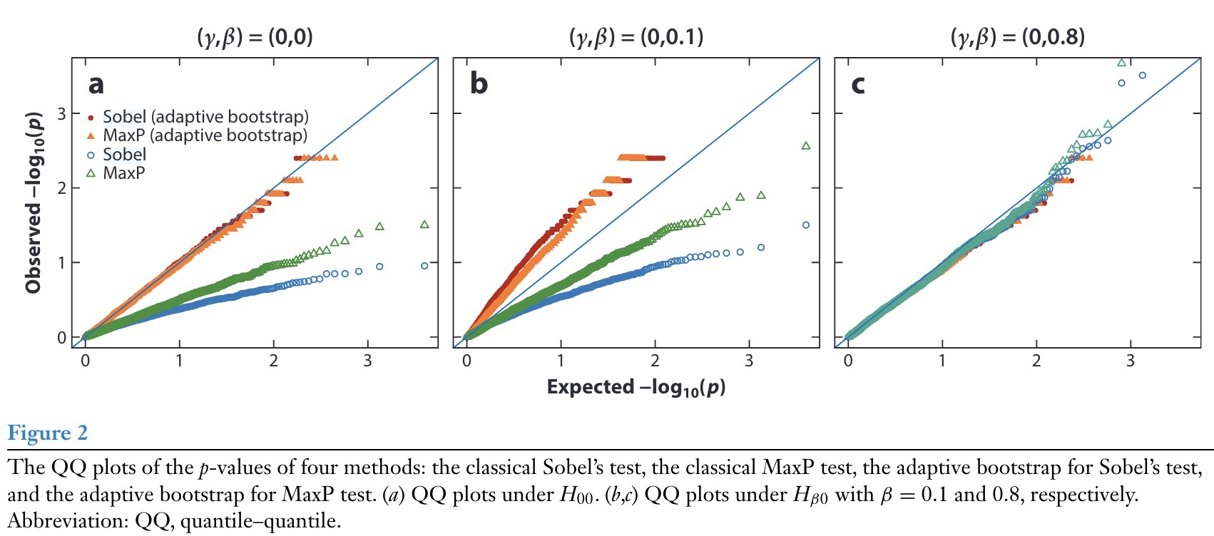
Yang’s notation \(\beta\) and \(\gamma\) refer to what we denoted as \(\theta_M\) and \(\beta_A\), respectively, \(\mathrm{H}_{\beta 0}\) is equivalent to \(\mathrm{H}_{01}\).
1.2 High-dimensional Mediation Hypothesis Testing
Now with the understanding that the \(\mathrm{MaxP}\) test is the most powerful test of univariate mediation, we return to the problem of testing \(p\) possible mediators under the model Equation 1. In the marginal mediation analysis framework, we assume the \(p\) mediators are in parallel, i.e. there is no causal ordering between mediators. Our proposed approach to for DNA methylation is to analyze individual mediators \(M^{(k)}\) one at a time across the epigenome and to select potential mediators by conducting a large number of mediation tests, adjusting for multiple comparisons.
The adjustment for multiple comparisons relies on being able to accurately estimate the probabilities of each case in the composite null hypothesis \(\mathrm{H}_0\).
\[ \begin{align} \pi_{01} &= \mathrm{Pr}\<[\beta_A^{(k)} = 0, \theta_M^{(k)} \neq 0\>]\\ \pi_{10} &= \mathrm{Pr}\<[\beta_A^{(k)} \neq 0, \theta_M^{(k)} = 0\>]\\ \pi_{00} &= \mathrm{Pr}\<[\beta_A^{(k)} = 0, \theta_M^{(k)} = 0\>] \end{align} \]
We assume \(\widehat{\beta}_A^{(k)}\) and \(\widehat{\theta}_M^{(k)}\) are independent. Then, by leveraging prior results on high-dimensional hypothesis testing, we can borrow information across the \(p\) mediators to estimate \(\pi_{\beta_A} = \mathrm{Pr}[\beta_A = 0]\) and \(\pi_{\theta_M} = \mathrm{Pr}[\theta_M = 0]\). Using these estimates, plug-in estimators of each of the probabilities of observing each null hypothesis are easily obtained,
\[ \begin{align} \widehat{\pi}_{01}^{(k)} &= \widehat{\pi}_{\beta_A}^{(k)} \times \<(1 - \widehat{\pi}_{\theta_M}^{(k)}\>)\\ \widehat{\pi}_{10}^{(k)} &= \<(1 - \widehat{\pi}_{\beta_A}^{(k)}\>) \times \widehat{\pi}_{\theta_M}^{(k)}\\ \widehat{\pi}_{01}^{(k)} &= \widehat{\pi}_{\beta_A}^{(k)} \times \widehat{\pi}_{\theta_M}^{(k)} \end{align} \]
Using this approach, (Liu et al. 2022) and (Dai, Stanford, and LeBlanc 2022) constructed the \(\mathrm{DACT}\) and \(\mathrm{HDMT}\) tests for multiple mediation.
1.2.1 Divide and Aggregate Composite Test (DACT)
For the \(k\)-th mediator \(M^{(k)}\), Liu proposed the DACT test statistic:
\[ T_{\mathrm{DACT}}^{(k)} = \widehat{\pi}_{10}^{(k)} p_{\beta_A}^{(k)} + \widehat{\pi}_{01}^{(k)} p_{\theta_M}^{(k)} + \widehat{\pi}_{00}^{(k)} \<(p_{\max}^{(k)}\>)^2 \]
When either \(\pi_{01}^{(k)}, \pi_{10}^{(k)}\) or \(\pi_{01}^{(k)}\) are close to \(1\), \(T_{\mathrm{DACT}}^{(k)}\) is uniformly distributed under the null. However, when this is not the case, \(T_{\mathrm{DACT}}\) has a complicated null distribution. Liu’s solution to this was to use the empirical null of an inverse-normal transformed statistic \(Z_{\mathrm{DACT}}\),
\[ Z_{\mathrm{DACT}}^{(k)} = \Phi^{-1}\<(1 - T_{\mathrm{DACT}}^{(k)}\>) \]
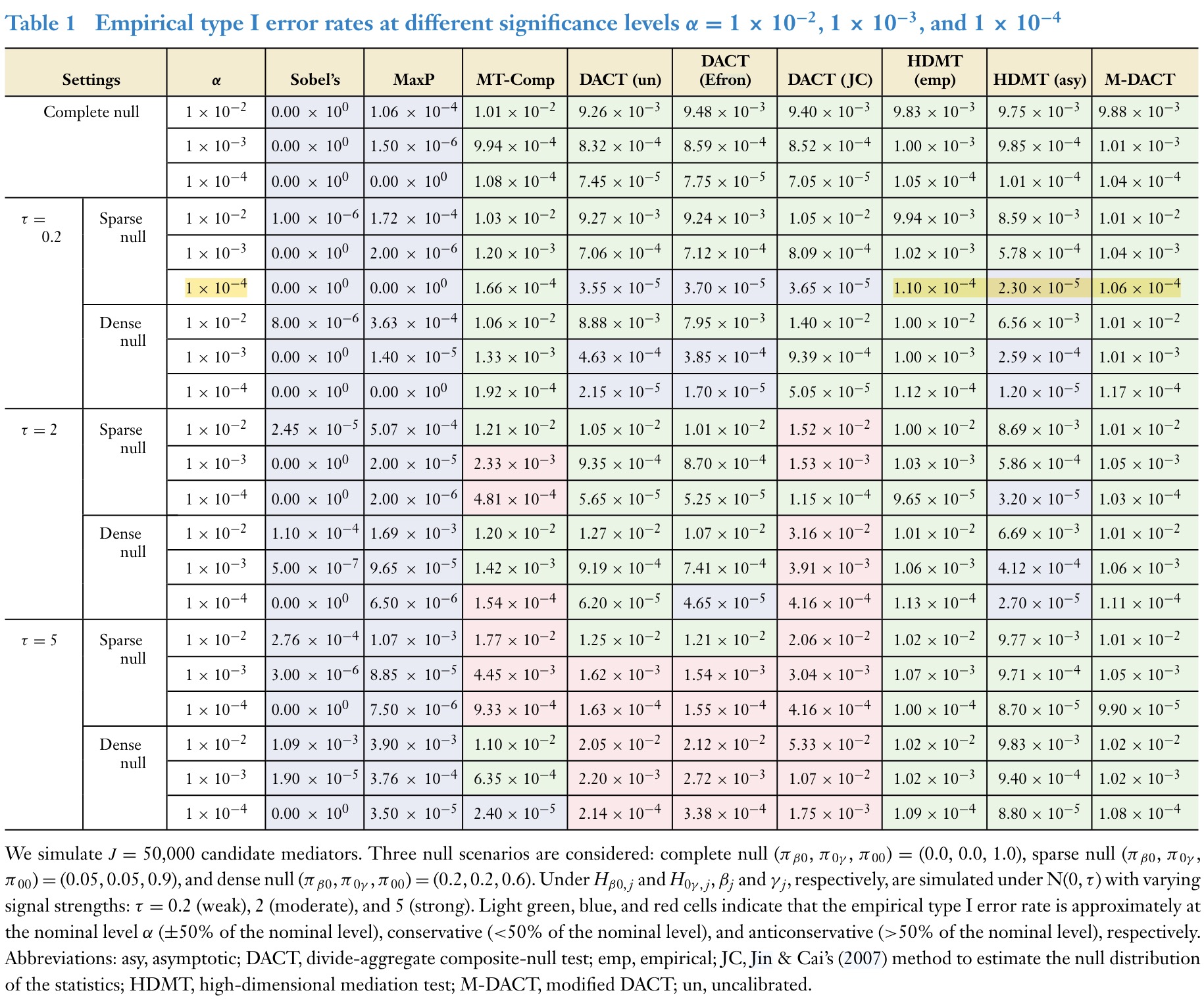
In simulations, Du (Du et al. 2023) and Yang (Yang et al. 2025) both showed that when \(\pi_{01}\) and \(\pi_{10}\) are common and the effect sizes are also large, \(\mathrm{DACT}\) fails to control Type-I error. Note, both Du and Yang only considered symmetric scenarios, where \(\beta_A^{(k)}\) and \(\theta_M^{(k)}\) were both large in magnitude. For our case, the mediation of the effect mean-HbA1c on the onset of diabetic retinopathy by DNA methylation seems to be highly asymmetric, many CpG sites are strongly associated with mean-HbA1c, but relatively few CpG sites are associated with time-to-retinopathy, with very weak signals.
1.2.1.1 modified-DACT
Yang identified DACT’s problems as being related to poor estimation of the empirical null of \(Z_{\mathrm{DACT}}\). As a remedy, he defined a procedure designed to estimate the empirical null of \(T_{\mathrm{DACT}}\) itself called \(\mathrm{M-DACT}\), with favorable simulation results. He considers the CDF of \(T_{\mathrm{DACT}}\) under the three conditional null hypotheses,
\[ \begin{align} \operatorname{Pr}\<[T_{\mathrm{DACT}}^{(k)} < t \mid \mathrm{H}_{0}^{(k)} \>] &= \operatorname{Pr}\<[T_{\mathrm{DACT}}^{(k)} < t \mid \mathrm{H}_{01}^{(k)}\>] \operatorname{Pr}\<[\mathrm{H}_{01}^{(k)}\>] \\ &\qquad+ \operatorname{Pr}\<[T_{\mathrm{DACT}}^{(k)} < t \mid \mathrm{H}_{10}^{(k)}\>] \operatorname{Pr}\<[\mathrm{H}_{10}^{(k)}\>]\\ &\qquad+ \operatorname{Pr}\<[T_{\mathrm{DACT}}^{(k)} < t \mid \mathrm{H}_{00}^{(k)}\>] \operatorname{Pr}\<[\mathrm{H}_{00}^{(k)}\>] \end{align} \]
and defines plug-in estimators for all six unknown probabilities. No code was provided.
1.2.2 High-Dimensional Mediation Testing (HDMT)
Similar to DACT, Dai’s HDMT (Dai, Stanford, and LeBlanc 2022) method requires estimating \(\pi_{01}\), \(\pi_{10}\), and \(\pi_{00}\), but he instead directly tried approximate the distribution of \(T_{\mathrm{MaxP}}\) under the composite null \(\mathrm{H}_0\).
\[ \begin{align} \operatorname{Pr}\<[T_{\mathrm{MaxP}}^{(k)} \leq t \mid \mathrm{H}_{0}^{(k)} \>] &= \operatorname{Pr}\<[T_{\mathrm{MaxP}}^{(k)} \leq t \mid \mathrm{H}_{01}^{(k)}\>] \operatorname{Pr}\<[\mathrm{H}_{01}^{(k)}\>] \\ &\qquad+ \operatorname{Pr}\<[T_{\mathrm{MaxP}}^{(k)}\leq t \mid \mathrm{H}_{10}^{(k)}\>] \operatorname{Pr}\<[\mathrm{H}_{10}^{(k)}\>]\\ &\qquad+ \operatorname{Pr}\<[T_{\mathrm{MaxP}}^{(k)}\leq t \mid \mathrm{H}_{00}^{(k)}\>] \operatorname{Pr}\<[\mathrm{H}_{00}^{(k)}\>]\\ &= \pi_{01} t \operatorname{Pr} \<[p_{\theta_M}^{(k)} \leq t \mid \mathrm{H}_{01} \>] \\ &\qquad+ \pi_{10} t \operatorname{Pr} \<[p_{\beta_A}^{(k)} \leq t\mid \mathrm{H}_{10} \>]\\ &\qquad+ \pi_{00} t^2\\ &= (\pi_{01} + \pi_{10}) t + \pi_{00} t^2 \end{align} \]
Note that \(\operatorname{Pr} \<[p_{\beta_A}^{(k)} \leq t \mid \mathrm{H}_{10} \>] \to 1\) and \(\operatorname{Pr} \<[p_{\theta_M}^{(k)} \leq t \mid \mathrm{H}_{01} \>] \to 1\), i.e. for large \(n\), the probability we reject the null that \(\beta_A = 0\), given \(\mathrm{H}_{10}\), goes to one. Thus, the asymptotic null distribution of \(T_{\mathrm{MaxP}}\) is a weighted mixture,
\[ \operatorname{Pr}\<[T_{\mathrm{MaxP}}^{(k)} \leq t \mid \mathrm{H}_{0}^{(k)} \>] = (\pi_{10} + \pi_{01})\operatorname{Pr}[\mathcal{U} \leq t] + \pi_{00} \operatorname{Pr}[\mathcal{F} \leq t] \]
where \(\mathcal{U}\) is uniformly distributed in the unit interval and \(\mathcal{F}\) is \(\mathrm{Beta}(2,1)\) distributed, since it is the maximum of two independent uniformly distributed variables. Using the characterization of the distribution of \(T_{\mathrm{MaxP}}\) under \(\mathrm{H}_0\), Dai constructs a FWER threshold and a method to control FDR.
He also develops finite sample adjusted procedures to control FWER and FDR, by defining estimators of the two power functions, \(\operatorname{Pr} \<[p_{\beta_A}^{(k)} \leq t \mid \mathrm{H}_{10} \>]\) and \(\operatorname{Pr} \<[p_{\theta_M}^{(k)} \leq t \mid \mathrm{H}_{01} \>]\)
1.2.2.1 Family-wise Error Rate Control
Given estimates \(\widehat{\pi}_{10}\), \(\widehat{\pi}_{01}\), and \(\widehat{\pi}_{00}\), the threshold to control the asymptotic family-wise error rate for a given \(\alpha\) can be derived easily, since,
\[ \operatorname{Pr}[T_{\mathrm{MaxP}} \leq t_{\alpha}] = \pi_{10} t_\alpha + \pi_{01} t_\alpha + \pi_{00} t_\alpha^2 \]
So given the nominal Bonferoni threshold \(\alpha / p\), the FWER threshold is the \(t_\alpha\) satisfying
\[ \frac{\alpha}{p} = \widehat{\pi}_{10} t_\alpha + \widehat{\pi}_{01} t_\alpha + \widehat{\pi}_{00} t_\alpha^2 \]
1.2.2.2 False Discovery Rate Control
When the number of mediation tests \(p\) is large, the false discovery rate associated with a test at level \(t\) can be estimated:
\[ \mathrm{FDR}(t) = \frac{\mathbb{E}\<[\text{number of rejected tests at level } t \mid \mathrm{H}_0 \>]}{ \mathbb{E}\<[\text{number of rejected tests at level } t \>]} \]
Then, by decomposing the composite null, we have,
\[ \begin{align} \mathrm{FDR}(t) &= \frac{\<(p \pi_{10} t + p \pi_{01} t + p \pi_{00}t^2 \>)}{ \mathbb{E}\<[\text{number of rejected tests at level } t \>]}\\ &\approx \frac{\<( \widehat{\pi}_{10} t + \widehat{\pi}_{01} t + \widehat{\pi}_{00}t^2 \>)}{ \frac{1}{p} \mathbb{E}\<[\text{number of rejected tests at level } t \>]} \end{align} \]
1.2.3 Yang (Yang et al. 2025) Simulations
1.3 Joint Mediation by Multiple Mediators
The natural direct effect (NDE) and total natural indirect effect (TNIE) are not identifiable by marginal mediation analysis using Equation 1. This is due to the fact that, in general, mediators driven by the same exposure are often correlated. For example, methylation at any pair of CpG sites \(\mathbf{m}_j\) and \(\mathbf{m}_k\). To correctly measure the joint mediation effect by all \(p\) mediators, we define the following model. Assuming that mediators are not causally related, let \(\mathbf{M} = \<[\mathbf{m}_1 \cdots \mathbf{m}_p \>]\). Then, the joint mediation model is,
\[ \begin{align} \mathbf{M} &= \mathbf{1}_n \boldsymbol{\beta}_0^\top + \mathbf{a} \boldsymbol{\beta}_A^\top + \mathbf{Z}_M \mathbf{B}_M + \mathbf{E}\\ \mathbf{y} &= \mathbf{1}_n \theta_0 + \mathbf{a} \theta_A + \sum_{j=1}^p \mathbf{m}_j \theta_{M,j} + \mathbf{Z}_Y \boldsymbol{\theta}_Y + \sigma \boldsymbol{\xi}\\ &= \mathbf{1}_n \theta_0 + \mathbf{a} \theta_A + \mathbf{M} \boldsymbol{\theta}_M + \mathbf{Z}_Y \boldsymbol{\theta}_Y + \sigma \boldsymbol{\xi} \end{align} \tag{2}\]
where \(\mathbf{E} \sim \mathrm{MN}(\mathbf{0}, \mathbf{I}_n, \boldsymbol{\Sigma})\). The estimate for the Natural Direct Effect is now identifiable since this formulation properly estimates the decomposition of total effect into direct and indirect effects, since \(\mathrm{TE} = \mathrm{NDE} + \mathrm{TNIE}\).
\[ \begin{align} \mathrm{NDE} &= \theta_A \\ \mathrm{TNIE} &= \sum_{j=1}^p \beta_{A,j} \theta_{M, j} = \boldsymbol{\beta}_A^\top \boldsymbol{\theta}_M\\ \end{align} \]
Furthermore, we can also express the proportion of the effect mediated.
\[ \begin{align} \mathrm{PM} = \frac{\mathrm{TNIE}}{\mathrm{NDE} + \mathrm{TNIE}} = \frac{\boldsymbol{\beta}_A^\top \boldsymbol{\theta}_M}{\theta_A + \boldsymbol{\beta}_A^\top \boldsymbol{\theta}_M} \end{align} \]
However, when the number of potential mediators exceeds the number of observations, \(p >> n\), the outcome model becomes a high-dimensional regression problem, having more parameters than observations. In practice, this does not seem to be a problem, since we use marginal mediation testing as a selection procedure before estimating the joint indirect effect. Given the large sample size in MVP, but this could present issues for replication analyses that have fewer samples.
There are more sophisticated approaches to the joint mediation problem that we briefly outline. Existing methods broadly fit into three general categories:
1.3.1 Dimension Reduction
Assuming that the \(p\) mediators \(\mathbf{m}_1, \dots, \mathbf{m}_p\) can be rotated in such a way such that the linearly transformed mediators \(\mathbf{u}_1, \dots, \mathbf{u}_p\) are both mutually linearly independent as well as orthogonal to the other covariates in the outcome model \(\mathbf{1}_n, \mathbf{a}\) and \(\mathbf{Z}_Y\). Then, the total mediation effect can be estimated by fitting \(p\) univariate mediation models: \[ \begin{align} \mathbf{u}_j &\sim \mathbf{1}_n \beta_{0, j} + \mathbf{a} \beta_{A, j} + \mathbf{Z}_M \boldsymbol{\beta}_{M, j} \\ \mathbf{y} &\sim \mathbf{1}_n \theta_{0, j} + \mathbf{a} \theta_{A, j} + \mathbf{Z}_Y \boldsymbol{\theta}_{Y, j} + \mathbf{u}_j \theta_{M, j} \end{align} \]
Let \(\mathbf{X} = \begin{bmatrix}\mathbf{1}_n & \mathbf{a} & \mathbf{Z}_Y & \mathbf{U}\end{bmatrix}\). Then, \[ \mathbf{X}^\top \mathbf{X} = \begin{bmatrix} n & \mathbf{1}_n^\top \mathbf{a} & \mathbf{1}_n^\top \mathbf{Z}_Y & \mathbf{0}_p^\top \\ \mathbf{1}_n^\top \mathbf{a} & \sum_i a_i^2 & \mathbf{a}^\top \mathbf{Z}_Y & \mathbf{0}_p^\top \\ \mathbf{Z}_Y^\top \mathbf{1}_n & \mathbf{Z}_Y^\top \mathbf{a} & \mathbf{Z}_Y^\top \mathbf{Z}_Y & \mathbf{0}_{q, p}\\ \mathbf{0}_p & \mathbf{0}_p & \mathbf{0}_{p,q} & \mathbf{U}^\top \mathbf{U} \end{bmatrix} \]
. The Schur complement is simply \(\mathbf{U}^\top \mathbf{U}\), which is diagonal by construction. Thus each \(\theta_{M, j}\) can be estimated marginally, allowing the summation of the terms to provide an unbiased estimate of the total indirect effect \(\sum_j \beta_{M, j} \theta_{M,j}\). Note that the point estimate of the direct effect is estimated in all \(p\) models, but uncertainty quantification in general, will not be correct. Importantly, this is only valid in linear models, nonlinear models (like the AFT model) typically involve weights \(\mathbf{w}\) that depend on regression coefficient estimates, breaking the indepenence structure.
1.3.2 Mediation by Latent Factors
Very similar to the dimension reduction approach, Derkach proposed a model assuming that the effect of \(A\) on \(Y\) mediated by \(\mathbf{m}_1 \dots, \mathbf{m}_p\) is through a low-dimensional set of independent factors \(\mathbf{f}_1, \dots, \mathbf{f}_d\), \(d << p\).
\[ \begin{align} \mathbf{M} &= \mathbf{1}_n \boldsymbol{\beta}_0^\top + \mathbf{F} \boldsymbol{\Lambda} + \mathbf{E}_M\\ \mathbf{F} &= \mathbf{a} \boldsymbol{\beta}_F^\top + \mathbf{Z}_F \mathbf{B}_F + \mathbf{E}_F\\ \mathbb{E}\<[\mathbf{y}\>] &= \mathbf{1}_n \theta_0 + \mathbf{a}\theta_A + \mathbf{F} \boldsymbol{\theta}_F + \mathbf{Z}_Y \boldsymbol{\theta}_Y \end{align} \]
where \(\mathbf{E}_F \sim \operatorname{MN(\mathbf{0}, \mathbf{I}_n, \mathbf{I}_d)}\), \(\mathbf{E}_M \sim \operatorname{MN}(\mathbf{0}, \mathbf{I}_n, \boldsymbol{\Psi}^2)\) and \(\boldsymbol{\Psi} = \operatorname{diag}(\psi_1^2, \dots, \psi_p^2)\). The total effect is given by \(\boldsymbol{\beta}_F^\top \boldsymbol{\theta}_F + \theta_A\).
1.3.3 Penalized Likelihood
Instead of maximizing the likelihood \(\ell \<(\boldsymbol{\theta};\, \mathbf{y}, \mathbf{a}, \mathbf{M}, \mathbf{Z}_Y\>)\), we deal with potentially high dimensional \(\mathbf{M}\) penalizing the negative log-likelihood,
\[ f(\boldsymbol{\theta}) = -\ell(\boldsymbol{\theta}) + p_{\lambda}(\boldsymbol{\theta}_M) \]
where \(p_\lambda(\cdot)\) is a penalty function with parameter \(\lambda\).
2 Average Marginal Effect Estimation
This pertains to EWAS analysis. One item of contention is that regression on the \(M\)-value scale has no biological interpretability. Let \(b\) denote methylation on the beta value scale \(b \in (0,1)\). The transformation from \(\beta\) scale to \(M\)-value scale is a scaled logit transformation.
\[ m = \log_2\left(\frac{b}{1-b}\right) \equiv \operatorname{logit}(b) \div \log(2) \]
The inverse-transform is,
\[ b = \frac{2^m}{1+2^m} \equiv \operatorname{logit}^{-1}(m \times \log(2)) \]
Fitting a linear model on the \(M\) scale, where \(A\) is the exposure of interest, we have,
\[ \begin{align} \mathbf{m} &= \beta_0 \mathbf{1}_n + \beta_A \mathbf{a} + \mathbf{Z}_M \boldsymbol{\beta}_M+ \boldsymbol{\varepsilon}\\ &= \mathbf{X}\boldsymbol{\beta} + \boldsymbol{\varepsilon} \end{align} \]
. Note that \(\widehat{\beta}_A \times \log(2)\) gives an estimate on the log-odds scale for a one-unit change in the exposure \(A\). However, log-odds and odds may be confusing for biological interpretation, we would like to know for a given CpG site, what is the percent change in methylation given an increase in exposure.
This is a case of a retransformation problem, a well-studied problem in classical statistics. Let \(h(x) = \frac{2^x}{1+2^x} \equiv \operatorname{logit}^{-1}(cx)\) where \(c=\log(2)\). First, we require an estimator of the expected methylation value on the beta scale for subject \(i\), conditional on the observed covariates \(\mathbf{x}_i = \{1, a_i, \mathbf{z}_M \}\).
\[ \begin{align} \mathbb{E}_\varepsilon\left[b_i \mid \mathbf{x}_i\right] &= \mathbb{E}_\varepsilon[h(m_i) \mid \mathbf{x}_i] \\ &= \mathbb{E}_\varepsilon[h(\beta_0 + \beta_A a_i + \mathbf{z}_{M, i} \boldsymbol{\beta}_M + \varepsilon_i)]\\ &= \int_{-\infty}^\infty h(\beta_0 + \beta_A a_i + \mathbf{z}_{M, i}^\top \boldsymbol{\beta}_M + \varepsilon) f(\varepsilon) \operatorname{d}\varepsilon\\ &= \mathbb{E}_\varepsilon [b_i \mid \mathbf{x}_i] \end{align} \]
Then, to get the estimated change in beta value for a change in exposure, we can simply linearize about the expectation to get the population-averaged marginal effect for subject \(i\).
\[ \begin{align} \mathrm{ME}_{a_i}^{\mathrm{pop}} = \frac{\partial}{\partial a_i} \mathbb{E}_{\varepsilon} [b_i \mid \mathbf{x}_i] &= \beta_A \operatorname{\mathbb{E}}_{\varepsilon}\left[h^{(1)} \left(\mathbf{x}_i^\top \boldsymbol{\beta} + \varepsilon \right)\right] \end{align} \]
We average over all observations and obtain an average marginal effect estimate on the beta-scale.
\[ \mathrm{AME}_a^{\mathrm{pop}} = \beta_A \frac{1}{n}\sum_{i=1}^n \EE_{\varepsilon} \<[ h^{(1)} \left(\mathbf{x}_i^\top \boldsymbol{\beta} + \varepsilon \right) \>] \]
Plugging in parameter estimates for \(\widehat{\boldsymbol{\beta}}\) and \(\widehat{\sigma}^2\), we can use Monte Carlo or quadrature methods to evaluate the expection.
It is possible to avoid Monte Carlo integration by fitting a generalized linear model directly on the beta-values (proportion scale) with a quasi-binomial model. This greatly simplifies marginal effect estimation, at the cost of increased computation during GLM estimation. Additionally, this requires fewer parametric assumptions than a similar Beta regression model, and is more robust to cases of mostly hyper or hypo-methylation.
2.1 Inference
For standard errors of the average (conditional) marginal effect estimate, we take a delta method approach, assuming small changes in the exposure \(A\).
\[ \widehat{\mathrm{AME}}_a = \sum_{i=1}^n h^{(1)}\<(\mathbf{x}_i^\top \widehat{\boldsymbol{\beta}}\>) \]
\[ \begin{align} \operatorname{\nabla}_{\boldsymbol{\beta}} \mathrm{ME}_{a_i} = \operatorname{\nabla}_{\boldsymbol{\beta}} g_i(\boldsymbol{\beta}) &= \operatorname{\mathbb{E}}_{\varepsilon}\left[h^{(1)} \left(\mathbf{x}_i^\top \boldsymbol{\beta} + \varepsilon \right)\right] \mathbf{e}_2\\ &\qquad + \beta_A \operatorname{\mathbb{E}}_{\varepsilon}\left[h^{(2)} \left(\mathbf{x}_i^\top \boldsymbol{\beta} + \varepsilon \right)\right] \mathbf{x}_i\\ &\approx \left[\frac{1}{K}\sum_{k=1}^K h^{(1)} \left(\mathbf{x}_i^\top \boldsymbol{\beta} + \varepsilon_k \right) \right] \mathbf{e}_2\\ &\qquad + \beta_A \left[ \frac{1}{K}\sum_{k=1}^K h^{(2)} \left(\mathbf{x}_i^\top \boldsymbol{\beta} + \varepsilon_k \right) \right] \mathbf{x}_i\\ &= \widehat{\operatorname{\nabla}_{\boldsymbol{\beta}}} \mathrm{ME}_{a_i} \end{align} \]
where \(\mathbf{e}_2\) denotes the vector with \(1\) at the second coordinate and zeros otherwise. Averaging over all subjects, we get the approximate variance,
\[ \widehat{\operatorname{Var}} \left[\widehat{\mathrm{AME}}_a\right] = \frac{1}{n} \sum_{i=1}^n \left(\widehat{\operatorname{\nabla}_{\boldsymbol{\beta}}} \mathrm{ME}_{a_i}\right)^\top \operatorname{Cov}[\widehat{\boldsymbol{\beta}}] \left(\widehat{\operatorname{\nabla}_{\boldsymbol{\beta}}} \mathrm{ME}_{a_i}\right) \]
Note, we can avoid expanding the derivatives of \(h\) by observing that it is simply a scaled inverse-logit function. There is a well known recursion for derivatives of the inverse logit that we can modify to obtain derivatives for the \(M\)-value to beta-value transform.
\[ \begin{align} h^{(0)}(x) &= h(x)\\ h^{(1)}(x) &= \log(2) h(x) (1 - h(x)) \\ h^{(2)}(x) &= \log^2(2) h(x) (1 - h(x)) (1 - 2 h(x)) \end{align} \]
2.2 Extra Figures
